
PREDICTING MONTHLY URBAN WATER DEMAND IN A CHANGING CLIMATE: A CASE STUDY OF CASABLANCA CITY, MOROCCO.
Journal: Water Conservation and Management (WCM)
Author: Ikram Samih, Dalila Loudyi
Print ISSN : 2523-5664
Online ISSN : 2523-5672
This is an open access article distributed under the Creative Commons Attribution License CC BY 4.0, which permits unrestricted use, distribution, and reproduction in any medium, provided the original work is properly cited
Doi: 10.26480/wcm.01.2025.113.119
Abstract
 The governance of urban areas now extends beyond managing population growth, as urban expansion has amplified cities’ susceptibility to climate change effects. As a result, urban water supply systems are under increasing pressure, highlighting the necessity for utility managers and policymakers to adopt sustainable demand management strategies to enhance water resource resilience. The aim of this paper is to model monthly water demand using the Principal Component Regression (PCR) method. The analysis is conducted over a seven-year dataset (2015–2021) and incorporates demographic and climatic variables specific to Casablanca, Morocco. Furthermore, projected climatic variables from the CMIP6 over Mediterranean regions under SSP1 -2.6 and SSP5-8.5 Pathways was driven in order to forecast monthly water demand for the near term. This research contributes to the development of adaptive strategies for urban planners, enabling them to anticipate future water demand and implement necessary measures to enhance sustainability assessments.
Keywords
Principal component regression; water demand forecasting; urban water management; IPCC; CMIP6; Shared Socioeconomic Pathways; Interactive atlas
1. INTRODUCTION
Water has become a challenge of global dimensions (Pahl-Wostl et al. 2013). Many researchers and policy makers have given attention on large water consumers as agriculture and industry, giving minor focus to the capacity of cities to manage the urban water cycle properly (Rockström et al. 2014). Urban water management (UWM) has recently received more consideration, in part due to the global Sustainable Development Goal on water of Agenda 2030 (SDG 6). The generally accepted approach to UWM aimed to create resilient, loveable, productive and sustainable cities and towns. Therefore, most of the existing strategies and measures has only blindly concentrated on developing new resources, generally non- conventional, in order to satisfy the constantly increasing demand of the principal resource. That is to say, in response to population growth, increase of densely inhabited areas, development of the economic conditions a parallel increase in the total water consumption has to be met. This paradigm has necessitated a shift towards incorporating both water supply interventions and demand management strategies to effectively address the constraints of limited water resources. Water demand management strategies involve implementing effective usage restrictions, introducing programs aimed at reducing consumption, optimizing supply processes, and developing sustainable alternative water sources (Adamowski and Karapataki, 2010). Among various approaches, forecasting water demand plays a crucial role in enhancing the efficiency and sustainability of water resource management. It facilitates informed decision-making, contributing to the effective operation and management of water supply systems while supporting their long-term planning and design (Bougadis et al., 2005).
Water demand forecasting can be categorized into three main classes based on the forecast horizon and periodicity: (i) short-term forecasting, (ii) medium-term forecasting, and (iii) long-term forecasting (Bougadis et al., 2005; Froelich, 2015). While there is no universally accepted definition for these classifications, several studies suggest that forecasts extending beyond two years are considered long-term, those ranging between three months and two years fall under medium-term forecasting, and forecasts covering less than three months are classified as short-term (Bougadis et al., 2005). Long-term forecasting models of urban water demand play a crucial role in shaping policies and strategies to ensure future water supply adequacy. Additionally, long-term projections support the development, planning, and design of new water infrastructure while aiding in the identification of effective water conservation measures (Babel et al., 2007; Ghiassi et al., 2008; Firat et al., 2009; Herrera et al., 2010; Haque et al., 2014). Conversely, medium-term forecasting is instrumental in guiding strategic investment decisions and planning for the expansion of existing water infrastructure, whereas short-term forecasting is primarily utilized for optimizing the operation and maintenance of water supply systems (Herrera et al., 2010; Jain and Ormsbee, 2002). Consequently, all forecasting timeframes are essential for enabling relevant authorities to manage water supply systems with greater efficiency and effectiveness.
Accurately forecasting water demand remains a complex and challenging task, influenced by various factors such as the type and quality of available data, the multiplicity of water demand variables, geographical variations across forecast regions, differences in forecasting horizons, and diverse demographic conditions. Numerous exogenous factors influence predictive models of urban water demand, either directly or indirectly. These factors range from climatic and meteorological conditions to the geographic characteristics of the study areas. Additionally, economic indicators, socio-demographic conditions, calendar-based variations, and technological advancements have been identified as significant variables in the development of urban water demand forecasting methods (Niknam et al., 2022). As a result, extensive research has been conducted to refine demand modeling approaches and improve forecasting tools, ultimately enhancing the overall accuracy and reliability of predictions.
A wide range of methods has been employed in water demand forecasting, including regression analysis time-series modeling and artificial neural networks (Salloom et al., 2021; Hu et al., 2021; Herrera et al., 2010; Haque et al., 2017; Bakker et al., 2014; Maruyama and Yamamoto, 2019; Rasifaghihi et al., 2020; Chen and Boccelli, 2014; Arandia et al., 2016; Ristow et al., 2021). Additionally, some studies have explored hybrid modeling approaches by integrating two or more methods to improve predictive accuracy (Herrera et al., 2011; Oliveira et al., 2017; Sardinha-Lourenço et al., 2018). Among these techniques, multiple linear regression (MLR) remains one of the most widely applied methods for water demand forecasting due to its relative simplicity and ease of interpretation (Adamowski and Karapataki, 2010). Various adaptations of MLR, including linear, log-linear, and log-log models, have been utilized in water demand modeling. In MLR applications, multiple influencing factors discussed earlier are incorporated into the model, either with or without logarithmic transformations.
Several studies have employed the principles of MLR techniques while modifying the selection of water demand variables, replacing original variables with alternative representations. Principal Component Regression (PCR) is a form of regression analysis that utilizes principal components (PCs) as independent variables instead of the original dataset (Pires et al., 2008). These PCs are derived as linear combinations of the original variables through Principal Component Analysis (PCA), which transforms a set of intercorrelated independent variables into a new set of uncorrelated components. By incorporating PCs as independent variables in multiple regression models, PCR effectively mitigates multicollinearity issues and identifies the most influential predictors for water demand management. For instance, applied both MLR and PCR techniques to predict the significant concentrations of seven environmental pollutants affecting the ozone layer (Abdul-Wahab et al., 2005). The research integrated a multiple regression model with PCA to enhance the prediction of urban water demand in Aquidauana, Mato Grosso do Sul (MS), (Brazil Ristow et al., 2021). When comparing the performance of PCR and MLR for both modeling and forecasting, PCR demonstrated superior accuracy in simulating water demand. These studies collectively highlight that incorporating PCs as independent variables not only improves predictive performance but also simplifies model complexity by eliminating multicollinearity.
This study seeks to explore, for the first time in Casablanca, Morocco, the application of the Principal Component Regression (PCR) method for short-term urban water demand forecasting. The primary goal is to determine the most influential variables in water demand modeling using PCR. Furthermore, the established PCR model is employed to forecast monthly water demand in Casablanca for the near-term period (2021–2040) based on projected explanatory variables.
2.STUDY AREA AND DATA
2.1 Study Area
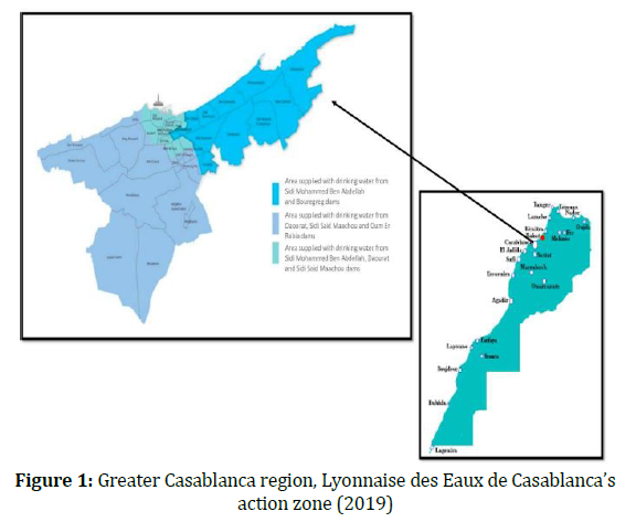
Casablanca, often referred to as the “White City,” is situated on the Atlantic coast of the Chaouia plain in the central-western region of Morocco. As the largest city in North Africa, it serves as Morocco’s economic and financial hub, recognized as a Global Financial Centre, ranking 53rd worldwide in the Global Financial Centers Index for 2021. With a population exceeding 4 million, Casablanca plays a significant role in national economic activity, particularly in household final consumption and value creation.
The interconnection between water resources and major urban centers is critical, as large cities require substantial freshwater inputs while exerting considerable pressure on freshwater systems. Sustainable urban development relies on ensuring reliable access to safe drinking water and adequate sanitation services. In this context, Lyonnaise des Eaux de Casablanca (Lydec) operates as the public service provider responsible for water and electricity distribution, wastewater and rainwater management, and public lighting across the Greater Casablanca region, encompassing Casablanca, Mohammedia, and Aïn Harrouda. However, this study focuses exclusively on Casablanca, as it is the most densely populated and urbanized city within the region.
Recently, Moroccan government imposed various water restrictions based on the substantial deficit in the last months of 2021 to ensure a rational management of the available water resources for the preservation of the resource and, to guarantee the supply of drinking water in satisfactory conditions in large cities such as Marrakesh and Casablanca (for instance, Casablanca registered an increase of 15% of residential consumption for the period of 2015-2021). The application of restrictions on the flow of water distributed to users was the most severe restrictions among the seven restrictions. Severely drier than normal conditions are forecasted at most watershed scale. These forecasts currently represent the principal concern, as they point to a possible evolution of the ongoing drought into an extreme event. Monitoring and managing such evolution in the next months are essential for risk and impact assessment, hence the strong need for our study.
2.2 Data
Water demand is influenced by a wide range of factors, which can generally be classified into two main categories: socioeconomic and climatic variables. Research indicates that socioeconomic factors primarily drive long-term trends in water consumption, whereas climatic variables predominantly account for short-term seasonal fluctuations in water demand (Miaou, 1990).
This study utilizes historical data on water consumption, demographic factors, and climatic variables. Specifically, the dataset includes monthly residential water consumption (m³), mean, maximum, and minimum temperatures (°C), wind speed (km/h), relative humidity (%), total population, and total rainfall (mm).
Water consumption data were obtained from Lyonnaise des Eaux de Casablanca, population data were sourced from the Haut Commissariat au Plan, and meteorological data were collected from the Direction de la Météorologie Nationale in Casablanca. The available water consumption records span from 2015 to 2021, representing the most comprehensive dataset at the time of the study, with the possibility of updates in the future. The projected climatic variables for the future period (2021–2040) were derived from the IPCC WGI Interactive Atlas: Regional Information (Advanced), based on data from the Coupled Model Intercomparison Project Phase 6 (CMIP6). These projections were generated for the Mediterranean region under the SSP1-2.6 and SSP5-8.5 scenarios.
3.METHODS AND STUDY DESIGN
In this section, we present the methodological approach applied in this study (Figure 2).
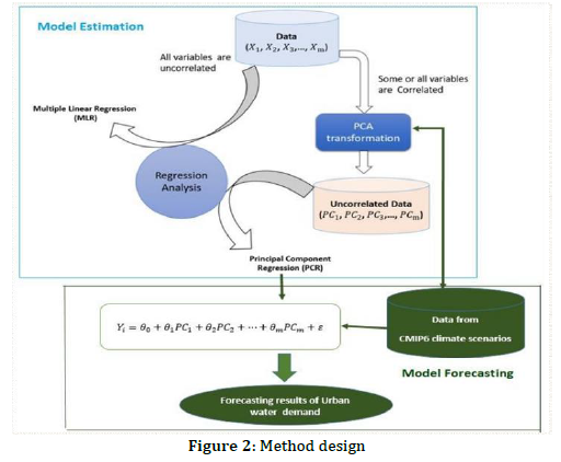
4.REGRESSION ANALYSIS
Regression analysis quantifies the linear relationship between a dependent variable (Y) and one or more explanatory variables (𝑋1, 𝑋2, …, 𝑋m). This technique facilitates the modeling of associations between selected variables and enables the prediction of values based on the derived equation. When employing the ordinary least squares (OLS) method, certain underlying assumptions must be validated to ensure the reliability and accuracy of the regression model.
𝑌𝑖 = 𝛽0 + 𝛽1𝑋1 + 𝛽2𝑋2 + ⋯ + 𝛽𝑚𝑋𝑚 + 𝜀 (Eq. 1)
• 𝑌𝑖 = observed value of the dependent variable at point/time i.
• 𝛽0 = intercept value, i.e intersection with the y-axis, the value of 𝑌𝑖 when 𝑋1 = 𝑋2 = ⋯ = 𝑋𝑚 = 0.
• 𝛽𝑖 = regression coefficient or slope for explanatory variable 𝑋 at point i, i.e
• 𝛽𝑖 = 𝑑𝑌𝑖.𝑑𝑋𝑖
• 𝜀 error component.
To ensure the validity of the Ordinary Least Squares (OLS) method, the following assumptions must be tested and confirmed:
• Linearity: The relationship between the dependent and independentvariables should be linear.
• Random Sampling: The data must be collected randomly to avoid bias.
• No Multicollinearity: Independent variables should not be highly correlated with each other
• Minimal Measurement Error: Explanatory variables should be measured accurately.
• Zero Mean of Residuals: The sum of the residuals should be close to zero.
• Constant Variance: Residuals should have equal variance across all levels of the independent variables (homoscedasticity).
• Normal Distribution of Residuals: Residuals should follow a normal distribution.
• No Autocorrelation: Residuals should not be correlated with each other over time.
4.1 Principal Component Analysis (PCA)
Principal Component Analysis (PCA) is a multidimensional descriptive technique, also referred to as a factorial method, that is applied to quantitative variables. Its main objective is to transform a set of correlated variables into a new set of uncorrelated variables, known as principal components (PC1, PC2, …, PCm). These principal components are derived as linear combinations of the original variables (𝑋1, 𝑋2, …, 𝑋m), allowing for dimensionality reduction while preserving the essential structure of the data.
𝑃𝐶1 = 𝛼11𝑋1 + 𝛼12𝑋2 … … + 𝛼1𝑚𝑋𝑚 = Σ𝑛 𝑎1𝑗𝑥𝑗
𝑃𝐶2 = 𝛼21𝑋1 + 𝛼22𝑋2 … … + 𝛼2𝑚𝑋𝑚 = Σ𝑛 𝑎2𝑗𝑥𝑗
𝑃𝐶i = Σ𝑚 𝛼i𝑗𝑋𝑗, for 𝑖 = 1, … , 𝑚 (Eq. 2)
𝛼ij are the eigenvalues extracted from the covariance or correlation matrix of the data set.
4.2 Principal Component Regression (PCR)
In Principal Component Regression (PCR) analysis, regression techniques are combined with Principal Component Analysis (PCA) to establish a relationship between the dependent variable Y and the transformed independent variables, known as principal components (PC1, PC2, …, PCm) or (Dim1, Dim2, …, Dimm). This transformation helps address multicollinearity issues by replacing the original correlated variables with uncorrelated components. The estimated PCR model is then expressed as follows:
𝑌𝑖 = 𝜃0 + 𝜃1𝑃𝐶1 + 𝜃2𝑃𝐶2 + ⋯ + 𝜃𝑚𝑃𝐶𝑚 + 𝜀 (Eq. 3)
where 𝜃𝑖 are the elasticity’s coefficients and 𝜀 is the error component.
In order to validate the quality of the estimated model, we used the squared correlation coefficient indicator:
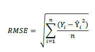
where 𝑌𝑖 is the observed value and 𝑌 𝑖 is the predicted or estimated value by the model.
4.3 Model Forecasting
A regression model utilizing temporal data enables the prediction of future values of the dependent variable Y, given that future values of some or all explanatory variables X are available for the selected prediction horizon. In this study, climate projections from CMIP6 were employed to estimate future urban water demand in Casablanca. The developed PCR model was applied to forecast average water consumption for the period 2022–2040, integrating projected climatic variables to analyze potential trends in water demand.
𝑌2022−2040 = 𝜃0 + 𝜃1𝑃𝐶12022−2040 + 𝑃𝐶22022−2040 + ⋯ + 𝜃𝑚𝑃𝐶𝑚2022−2040 + 𝜀 (Eq. 4)
Where;
𝑌2022−2040 is the average forecasted urban water demand over the period 2022-2040.
𝑃𝐶𝑖2022−2040 is the constructed principal component based on CMIP6 scenarios data.
5.RESULTS AND DISCUSSION
Following data collection, a correlation coefficient matrix was generated using SPSS software, as presented in Table 1. Statistically significant correlation coefficients (ρ < 0.05) are marked with stars. These coefficients help identify the strength of the linear relationship between variables and detect potential collinearity among independent variables, which is crucial for ensuring the reliability of the regression model.
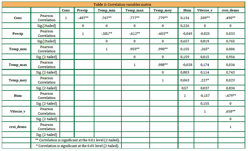
From Table 1, Cons exhibited a negative correlation with Precip, which aligns with expectations since higher precipitation reduces the need for water consumption, leading to lower residential water demand. Additionally, significant positive correlations were observed between key variables, such as Cons and Temp_moy (0.779), Vitesse_v and croi_demo (0.658), and Cons and Vitesse_v (0.509). These findings suggest the presence of multicollinearity among the selected variables, which may affect the reliability of regression estimates and necessitates the application of techniques such as Principal Component Analysis (PCA) to mitigate collinearity issues.
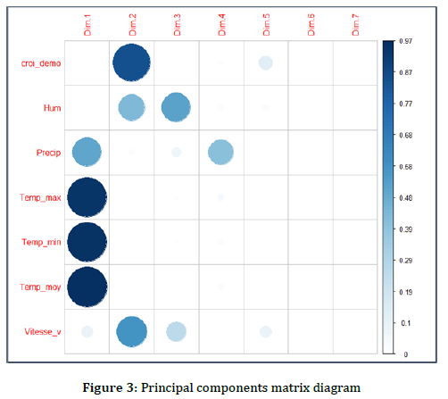
Principal Component Analysis (PCA) was conducted on seven independent variables to address multicollinearity and reduce dimensionality while preserving the essential information. Each principal component (PC) retains the overall variance of the original variables, ensuring that critical data patterns are maintained. The eigenvalues corresponding to each principal component are presented in Figure 3, which aids in selecting the most relevant components and understanding the dataset’s structure.
In the matrix diagram, the size of the colored disk represents the contribution of each variable to the corresponding principal component, with larger disks indicating a higher contribution. The analysis revealed that the first principal component (PC1) was predominantly influenced by climatic variables, particularly temperature and precipitation, while the second principal component (PC2) was primarily associated with demographic factors.
As shown in Table 2, the first four principal components were retained, accounting for 96.33% of the total variance in the dataset. These four PCs were selected to develop the Principal Component Regression (PCR) model, ensuring a comprehensive representation of the underlying data structure while minimizing redundancy.
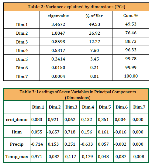
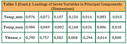
The influence of each independent variable within a principal component(PC) is determined by its component loading value, where higher absolutevalues (closer to 1 or -1) signify a stronger association with thecorresponding component. The sign of the loading (+ or -) indicateswhether the relationship between the variable and the principalcomponent is positive or negative. As shown in Table 3, the first principalcomponent (Dim.1), which accounts for 49.53% of the total variance,shows a strong negative loading for Precip (-0.714) and high positiveloadings for Temp_min (0.976), Temp_max (0.971), and Temp_moy(0.984). This suggests that Dim.1 is predominantly influenced bytemperature variables, reflecting the impact of urban climate conditions.The second principal component (Dim.2), explaining 26.92% of the totalvariance, is strongly associated with croi_demo (0.921) and shows notableloadings for Hum (-0.657) and Vitesse_v (0.757). Furthermore, the thirdand fourth principal components (Dim.3 and Dim.4) are mainlydetermined by Hum and Precip, respectively. These results indicate thatthe first two components capture the majority of the variance in thedataset, with Dim.1 representing climatic factors and Dim.2 reflecting thecombined influence of demographic and atmospheric variables.
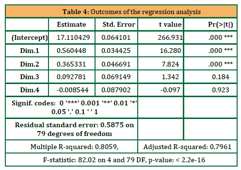
To calculate the principal component (PC) scores, the component scorecoefficients (eigenvectors) were multiplied by the values of the originalvariables. These scores were then used as independent variables in themultiple linear regression to identify the most influential PCs forpredicting water demand. Data from January 2015 to December 2021 wereutilized to construct the PCR model. As indicated in Table 4, the first fourprincipal components (i.e., Dim.1, Dim.2, Dim.3, and Dim.4) accounted forapproximately 80.59% of the variation in residential water consumption.Among these, Dim.1 and Dim.2 were found to be the most significantindependent variables in the PCR analysis (p-value < 0.000), both having apositive impact on urban water consumption. Specifically, an increase ofone unit in Dim.1 (comprising Precip, Temp_max, Temp_min, andTemp_moy) and Dim.2 (comprising croi_demo, Hum, and Vitesse_v) wouldresult in a predicted increase of 0.56 Mm³ and 0.3 Mm³ in residential waterconsumption, respectively. The resulting PCR model can be expressed asfollows:
𝐶𝑜𝑛𝑠𝑊 = 17.11 + 0.56 × 𝐷𝑖𝑚. 1 + 0.37 × 𝐷𝑖𝑚. 2 + 0.09 × 𝐷𝑖𝑚. 3 − 0.008 × 𝐷𝑖𝑚. 4 (Eq. 5)
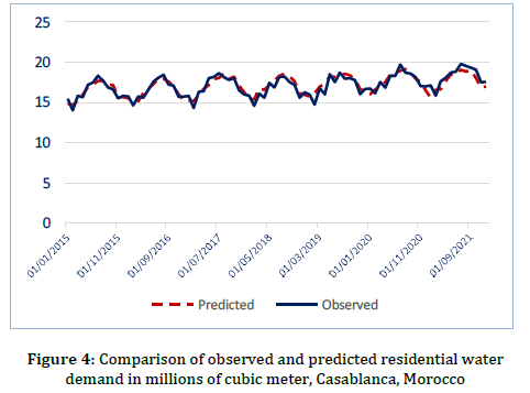
A comparison between the observed and modeled monthly residentialwater demand using the PCR model is shown in Fig. 4. The simulated valuesfor monthly water demand in the residential sector closely align with theobserved data. However, some discrepancies were noted in certainmonths, which could be attributed to significant fluctuations intemperature and rainfall, as well as potential changes in waterconsumption patterns. A daily demand model might capture thesevariations more effectively. Nonetheless, the Root Mean Square Error(RMSE) for all forecasted months was only 0.57 for residential waterconsumption, indicating that the developed model is highly accurate andsuitable for predicting both monthly and overall water demand.
The developed models can be utilized to forecast water demand for futuremonths in Casablanca, provided the predictor variable data are available(Eq. 1). However, if these predictor variables are not accessible, the modelscannot be applied directly. In this study, the IPCC Sixth Assessment Report(AR6) from Working Group I (WGI) interactive atlas—advanced regionalinformation—was used to generate aggregated tables for various keyvariables, as defined in the PCR model, for the Mediterranean region. Theseprojections were based on near-term scenarios under the weaker forcingscenario (SSP1-2.6) and the stronger forcing scenario (SSP5-8.5),representing the range of potential future climate trajectories.
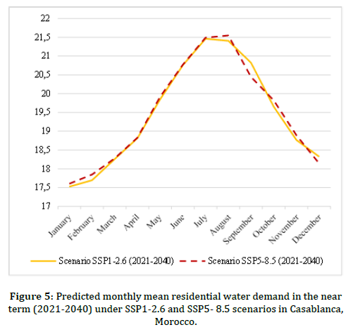
The projections obtained from Figure 5 for both scenarios indicate highervalues compared to the current situation, primarily due to changes in keypredictor variables defined in the PCR model (Eq. 1), such as temperature.The residential water demand will increase from 205 Mm3 (2015-2021) toaround 234 Mm3 as a mean value over the period of 2021-2040 under thestrongest scenario. This could capture a serious net increase of urbanwater requirements during each year of the selected forecasted period.This growth rate is estimated at around 1.6 Million m3 per year. Theprojection values of SSP5–8.5 scenario is approximately higher than theones from SSP1-2.6 scenario and from the current state except forSeptember and December, highlighting the importance that small changeson average monthly predicted PCs (Dim.1 and Dim.2) can cause majorchanges in the water demand. In Casablanca, forecasted residential waterdemand peaks during the summer months, and peak summer demandoccurs in August (21.54 Million m3 under SSP5–8.5 scenario). However,what may go unmentioned is the increased variability in summer monthdemands. As we can see from Figure 5, the average predicted residentialwater demand during summer months (June- August) rises by 16% incomparison of the average winter months (December-February)residential water demand.
The ability to accurately forecast water demand is crucial for the effective operation of water utilities. The preparedness of the full infrastructure, including both water treatment and distribution systems, plays a significant role in determining water pricing. Therefore, it is essential for water utilities to have access to detailed and precise water demand forecasts. Short-term monthly forecasts are particularly important for ensuring the efficient operation of the waterworks system, especially in minimizing the time that water spends in pipelines and reservoirs, which directly affects water quality. In cities like Casablanca and other major Moroccan urban centers, this becomes even more critical due to the rising water demand observed in recent years. As a result, hydraulic conditions in the water distribution system have changed, posing a serious threat to water quality, which can vary seasonally. By using accurate forecasting models, water distribution processes can be optimized, ensuring proper water quality, reducing risks, and enhancing the overall reliability of the water supply system, from the water intakes to households.
6.CONCLUSION
As populations and urban areas continue to grow, effective urban planning and sustainable water resource management are becoming increasingly essential. This study aims to highlight the importance of predicted urban water models in addressing future water scarcity issues, offering valuable insights for decision-makers, water managers, and land planners. A deeper understanding of the factors that alleviate future water shortages can help local and regional planners identify policy solutions that enhance the efficiency of water use moving forward.
Overall, the following key conclusions can be drawn:
• Seven Seven dependent variables were reduced to two key principal components through PCA, which together explained 76.46% of the total variance in the original dataset.
• PCR model shows important accuracy for residential monthly water-demand forecasting in Casablanca with capacity of prediction near to 80% (𝑅2 = 0.8).
• In reference to the developed PCR model, water demand in Casablanca city is predicted to increase, reaching a mean value of 234 millions of cubic meter with a peak water demand of 24.54 millions of cubic meter over the period of 2021-2040 under SSP5-8.5 scenario
The primary innovative contribution of this work is the development, for the first time in Morocco, of a Principal Component Regression (PCR) model to forecast water demand in Casablanca. This model incorporates predicted variables from the latest phase (Phase 6) of the CMIP, generated online via the IPCC WGI Interactive Atlas: Regional Information (Advanced) for the Mediterranean region, under the SSP1-2.6 and SSP5-8.5 scenarios.
REFERENCES
Abdul-Wahab, S.A., Bakheit, C.S., Al-Alawi, S.M., 2005. Principal component and multiple regression analysis in modelling of ground-level ozone and factors affecting its concentrations.Environmental Modelling and Software. 20(10): Pp. 1263-1271.
Adamowski, J., Karapataki, C., 2010. Comparison of Multivariate Regression and Artificial Neural Networks for Peak Urban Water-Demand Forecasting: Evaluation of Different ANN Learning Algorithms. Journal of Hydrologic Engineering, 15(10):Pp. 729–743. doi:10.1061/(asce)he.1943- 5584.0000245.
Arandia, E., Ba, A., Eck, B., McKenna, S., 2016. Tailoring seasonal time series models to forecast short- term water demand. J. Water Resour. Plan. Manag. 142:04015067.
Babel, M., Gupta, A.D., Pradhan, P., 2007. A multivariate econometric approach fo domestic water demand modeling: an application to Kathmandu, Nepal. Water Resour Manag. 21(3): Pp. 573–589
Bakker, M., Van Duist, H., Van Schagen, K., Vreeburg, J., Rietveld, L., 2014. Improving the performance of water demand forecasting models by using weather input. Procedia Eng. 70: Pp. 93–102.
Bougadis, J., Adamowski, K., and Diduch, R., 2005. Short-term municipal water demand forecasting.Hydrol. Process., 19: Pp. 137-148. https://doi.org/10.1002/hyp.5763
Chen, J., Boccelli, D., 2014. Demand forecasting for water distribution systems. Procedia Eng. 70: Pp. 339–342.
Donkor, E.A., Mazzuchi, T.A., Soyer, R., Alan Roberson, J., 2014. Urban Water Demand Forecasting: Review of Methods and Models. Journal of Water Resources Planning and Management, 140(2): Pp. 146–159. doi: 10.1061/ (asce)wr.1943-5452.0000314
First, M., Turan, M.E., Yurdusev, M.A., 2009. Comparative analysis of fuzzy inference systems for water consumption time series prediction. J. Hydrol. 374(3): Pp. 235–241
Froelich, W., 2015. Forecasting Daily Urban Water Demand Using Dynamic Gaussian Bayesian Network.In:
Kozielski, S., Mrozek, D., Kasprowski, P., Małysiak-Mrozek, B., Kostrzewa, D., 2015. (eds) Beyond Databases, Architectures and Structures. BDAS 2015. Communications in Computer and Information Science, 521. Springer, Cham. https://doi.org/10.1007/978-3-319-18422-7_30
Ghiassi, M., Zimbra, D.K., Saidane, H., 2008. Urban water demand forecasting with a dynamic artificial neural network model. J Water Resour Plan Manag.
Haque, M.M., de Souza, A., Rahman, A., 2017. Water demand modelling using inde pendent component regression technique. Water Resour. Manag. 31: Pp. 299–312
Haque, M.M., Rahman, A., Hagare, D., Kibria, G., 2014. Probabilistic water demand forecasting using projected climatic data for Blue Mountains water supply system in Australia. Water Resour Manag. 28(7): Pp. 1959–1971
Herrera, M., Torgo, L., Izquierdo, J., Pérez-García, R., 2010. Predictive models for forecasting hourly urban water demand. J Hydrol 387(1): Pp. 141–150
Herrera. M., García-Díaz, J.C., Izquierdo, J., Pérez-García, R., 2011. Municipal water demand forecasting: Tools for intervention time series. Stoch. Anal. Appl., 29, Pp. 998–1007.
Hu, S., Gao, J., Zhong, D., Deng, L., Ou, C., Xin, P., 2021. An innovative hourly water demand forecasting preprocessing framework with local outlier correction and adaptive decomposition techniques. Water. 13: Pp. 582.
Jain, A., Ormsbee, L.E., 2002. Short-term water demand forecast modeling techniques—Conventional methods versus AI. J Am Water Works Assoc. Pp. 64–72
Maruyama, Y., Yamamoto, H., 2019. A study of statistical forecasting method concerning water demand.Procedia Manuf. 39: Pp. 1801–1808.
Miaou, S., 1990. A class of time series urban water demand models with non-linear climatic effects. Water Resour. Res. 26(2): Pp. 169–178.
Niknam, A., Khademi Zare, H., Hosseininasab, H., Mostafaeipour, A., Herrera Fernandez, M.H., 2022. A critical review of short-term water demand forecasting tools. What method should I use? Sustainability.https://doi.org/10.17863/CAM.84047
Okeya I, Kapelan Z, Hutton C, Naga D. 2014. Online modelling of water distribution system using data assimilation. Procedia Eng. 70: Pp. 1261–1270
Oliveira, P.J., Steffen, J.L., Cheung, P., 2017. Parameter estimation of seasonal ARIMA models for water demand forecasting using the Harmony Search Algorithm. Procedia Eng. 186: Pp. 177–185.
Pires, J., Martins, F., Sousa, S., Alvim-Ferraz, M., Pereira, M., 2008. Selection and validation of parameters in multiple linear and principal component regressions. Environmental Modelling and Software. 23(1): Pp. 50-55.
Pahl-Wostl, C., Vörösmarty, C., Bhaduri, A., Bogardi, J., Rockström, J., Alcamo, J., 2013. Towards a sustainable water future: shaping the next decade of global water research. Current Opinion in Environmental Sustainability, 5(6): Pp. 708–714. doi:10.1016/j.cosust.2013.10.012
Rasifaghihi, N., Li, S., Haghighat, F., 2020. Forecast of urban water consumption under the impact of climate change. Sustain. Cities Soc. 52:101848
Ristow, D.C., Henning, E., Kalbusch, A., Petersen, C.E., 2021. Models for forecasting water demand using time series analysis: A case study in Southern Brazil. J. Water Sanit. Hyg. Dev. 11: Pp. 231–240.
Rockström, J., Falkenmark, M., Allan, T., Folke, C., Gordon, L., Jägerskog, A., Kummu, M., Lannersta, M., Meybeck, M., Molden, D., Postel, S., Savenije, H., Svedin, U., Turton, A., and Varis, O., 2014. The unfolding water drama in the Anthropocene: towards a resilience-based perspective on water for global sustainability, Ecohydrol., 7: Pp. 1249–1261, doi: 10.1002/eco.1562.
Salloom, T., Kaynak, O., He, W., 2021. A novel deep neural network architecture for real-time water demand forecasting. J. Hydrol. 599:126353.
Sardinha-Lourenço, A., Andrade-Campos, A., Antunes, A., Oliveira, M., 2018. Increased performance in the short-term water demand forecasting through the use of a parallel adaptive weighting strategy. J. Hydrol. 558, Pp. 392–404.
| Pages | 113-119 |
| Year | 2025 |
| Issue | 1 |
| Volume | 9 |
